Section4.2Estimating Area: Riemann Sums and Numerical Integration
Motivating Questions
How can we use a Riemann sum to estimate the area between a given curve and the horizontal axis over a particular interval?
What are the differences among left, right, middle, and random Riemann sums?
How can we write Riemann sums in an abbreviated form?
Are there ways to generate accurate estimates without using extremely large values of \(n\) in Riemann sums?
What is the Trapezoid Rule, and how is it related to left, right, and middle Riemann sums?
How are the errors in the Trapezoid Rule and Midpoint Rule related, and how can they be used to develop an even more accurate rule?
In Section 4.1, we learned that if an object moves with positive velocity \(v\text{,}\) the area between \(y = v(t)\) and the \(t\)-axis over a given time interval tells us the distance traveled by the object over that time period. If \(v(t)\) is sometimes negative and we view the area of any region below the \(t\)-axis as having an associated negative sign, then the sum of these signed areas tells us the moving object’s change in position over a given time interval.
For instance, for the velocity function given in Figure 4.2.1, if the areas of shaded regions are \(A_1\text{,}\)\(A_2\text{,}\) and \(A_3\) as labeled, then the total distance \(D\) traveled by the moving object on \([a,b]\) is
\begin{equation*}
D = A_1 + A_2 + A_3\text{,}
\end{equation*}
while the total change in the object’s position on \([a,b]\) is
Figure4.2.1.A velocity function that is sometimes negative.
Because the motion is in the negative direction on the interval where \(v(t) \lt 0\text{,}\) we subtract \(A_2\) to determine the object’s total change in position.
Of course, finding \(D\) and \(s(b)-s(a)\) for the graph in Figure 4.2.1 presumes that we can actually find the areas \(A_1\text{,}\)\(A_2\text{,}\) and \(A_3\text{.}\) So far, we have worked with velocity functions that were either constant or linear, so that the area bounded by the velocity function and the horizontal axis is a combination of rectangles and triangles, and we can find the area exactly. But when the curve bounds a region that is not a familiar geometric shape, we cannot find its area exactly. Indeed, this is one of our biggest goals in Chapter 4: to learn how to find the exact area bounded between a curve and the horizontal axis for as many different types of functions as possible.
In Activity 4.1.2, we approximated the area under a nonlinear velocity function using rectangles. In the following preview activity, we consider three different options for the heights of the rectangles we will use.
Preview Activity4.2.1.
A person walking along a straight path has her velocity in miles per hour at time \(t\) given by the function \(v(t) = 0.25t^3-1.5t^2+3t+0.25\text{,}\) for times in the interval \(0 \le t \le 2\text{.}\) The graph of this function is also given in each of the three diagrams in Figure 4.2.2.
Figure4.2.2.Three approaches to estimating the area under \(y = v(t)\) on the interval \([0,2]\text{.}\)
Note that in each diagram, we use four rectangles to estimate the area under \(y = v(t)\) on the interval \([0,2]\text{,}\) but the method by which the four rectangles’ respective heights are decided varies among the three individual graphs.
How are the heights of rectangles in the left-most diagram being chosen? Explain, and hence determine the value of
Of the estimates \(S\text{,}\)\(T\text{,}\) and \(U\text{,}\) which do you think is the best approximation of \(D\text{,}\) the total distance the person traveled on \([0,2]\text{?}\) Why?
Subsection4.2.1Sigma Notation
We have used sums of areas of rectangles to approximate the area under a curve. Intuitively, we expect that using a larger number of thinner rectangles will provide a better estimate for the area. Consequently, we anticipate dealing with sums of a large number of terms. To do so, we introduce sigma notation, named for the Greek letter \(\Sigma\text{,}\) which is the capital letter \(S\) in the Greek alphabet.
We read the symbol \(\sum_{k=1}^{100} k\) as “the sum from \(k\) equals 1 to 100 of \(k\text{.}\)” The variable \(k\) is called the index of summation, and any letter can be used for this variable. The pattern in the terms of the sum is denoted by a function of the index; for example,
Sigma notation allows us to vary easily the function being used to describe the terms in the sum, and to adjust the number of terms in the sum simply by changing the value of \(n\text{.}\) We test our understanding of this new notation in the following activity.
Activity4.2.2.
For each sum written in sigma notation, write the sum long-hand and evaluate the sum to find its value. For each sum written in expanded form, write the sum in sigma notation.
\(\displaystyle \sum_{k=1}^{5} (k^2 + 2)\)
\(\displaystyle \sum_{i=3}^{6} (2i-1)\)
\(\displaystyle 3 + 7 + 11 + 15 + \cdots + 27\)
\(\displaystyle 4 + 8 + 16 + 32 + \cdots + 256\)
\(\displaystyle \sum_{i=1}^{6} \frac{1}{2^i}\)
Subsection4.2.2Riemann Sums
When a moving body has a positive velocity function \(y = v(t)\) on a given interval \([a,b]\text{,}\) the area under the curve over the interval gives the total distance the body travels on \([a,b]\text{.}\) We are also interested in finding the exact area bounded by \(y = f(x)\) on an interval \([a,b]\text{,}\) regardless of the meaning or context of the function \(f\text{.}\) For now, we continue to focus on finding an accurate estimate of this area by using a sum of the areas of rectangles. Unless otherwise indicated, we assume that \(f\) is continuous and non-negative on \([a,b]\text{.}\)
The first choice we make in such an approximation is the number of rectangles.
Figure4.2.3.Subdividing the interval \([a,b]\) into \(n\) subintervals of equal length \(\Delta x\text{.}\)
If we desire \(n\) rectangles of equal width to subdivide the interval \([a,b]\text{,}\) then each rectangle must have width \(\Delta x = \frac{b-a}{n}\text{.}\) We let \(x_0 = a\text{,}\)\(x_n = b\text{,}\) and define \(x_{i} = a + i\Delta x\text{,}\) so that \(x_1 = x_0 + \Delta x\text{,}\)\(x_2 = x_0 + 2 \Delta x\text{,}\) and so on, as pictured in Figure 4.2.3.
We use each subinterval \([x_i, x_{i+1}]\) as the base of a rectangle, and next choose the height of the rectangle on that subinterval. There are three standard choices: we can use the left endpoint of each subinterval, the right endpoint of each subinterval, or the midpoint of each. These are precisely the options encountered in Preview Activity 4.2.1 and seen in Figure 4.2.2. We next explore how these choices can be described in sigma notation.
Consider an arbitrary positive function \(f\) on \([a,b]\) with the interval subdivided as shown in Figure 4.2.3, and choose to use left endpoints. Then on each interval \([x_{i}, x_{i+1}]\text{,}\) the area of the rectangle formed is given by
Figure4.2.4.Subdividing the interval \([a,b]\) into \(n\) subintervals of equal length \(\Delta x\) and approximating the area under \(y = f(x)\) over \([a,b]\) using left rectangles.
If we let \(L_n\) denote the sum of the areas of these rectangles, we see that
Note that since the index of summation begins at \(0\) and ends at \(n-1\text{,}\) there are indeed \(n\) terms in this sum. We call \(L_n\) the left Riemann sum for the function \(f\) on the interval \([a,b]\text{.}\)
To see how the Riemann sums for right endpoints and midpoints are constructed, we consider Figure 4.2.5.
Figure4.2.5.Riemann sums using right endpoints and midpoints.
For the sum with right endpoints, we see that the area of the rectangle on an arbitrary interval \([x_i, x_{i+1}]\) is given by \(B_{i+1} = f(x_{i+1}) \cdot \Delta x\text{,}\) and that the sum of all such areas of rectangles is given by
so that \(\overline{x}_{i+1}\) is the midpoint of the interval \([x_i, x_{i+1}]\text{.}\) For instance, for the rectangle with area \(C_1\) in Figure 4.2.5, we now have
and we say that \(M_n\) is the middle Riemann sum for \(f\) on \([a,b]\text{.}\)
Thus, we have two variables to explore: the number of rectangles and the height of each rectangle. We can explore these choices dynamically, and this applet 1
gvsu.edu/s/a9
is a particularly useful one. There we see the image shown in Figure 4.2.6, but with the opportunity to adjust the slider bars for the heights and the number of rectangles.
Figure4.2.6.A snapshot of the applet found at gvsu.edu/s/a9.
By moving the sliders, we can see how the heights of the rectangles change as we consider left endpoints, midpoints, and right endpoints, as well as the impact that a larger number of narrower rectangles has on the approximation of the exact area bounded by the function and the horizontal axis. We can also adjust the formula for \(f(x)\) and the window of \(x\)- and \(y\)-values of interest.
When \(f(x) \ge 0\) on \([a,b]\text{,}\) each of the Riemann sums \(L_n\text{,}\)\(R_n\text{,}\) and \(M_n\) provides an estimate of the area under the curve \(y = f(x)\) over the interval \([a,b]\text{.}\) We also recall that in the context of a nonnegative velocity function \(y = v(t)\text{,}\) the corresponding Riemann sums approximate the distance traveled on \([a,b]\) by a moving object with velocity function \(v\text{.}\)
There is a more general way to think of Riemann sums, and that is to allow any choice of where the function is evaluated to determine the rectangle heights. Rather than saying we’ll always choose left endpoints, or always choose midpoints, we simply say that a point \(x_{i+1}^*\) will be selected at random in the interval \([x_i, x_{i+1}]\) (so that \(x_i \le x_{i+1}^* \le x_{i+1}\)). The Riemann sum is then given by
\begin{equation*}
f(x_1^*) \cdot \Delta x + f(x_2^*) \cdot \Delta x + \cdots + f(x_{i+1}^*) \cdot \Delta x + \cdots + f(x_n^*) \cdot \Delta x = \sum_{i=1}^{n} f(x_i^*) \Delta x\text{.}
\end{equation*}
and referenced in Figure 4.2.6, by unchecking the “relative” box at the top left, and instead checking “random,” we can easily explore the effect of using random point locations in subintervals on a Riemann sum. In computational practice, we most often use \(L_n\text{,}\)\(R_n\text{,}\) or \(M_n\text{,}\) while the random Riemann sum is useful in theoretical discussions. In the following activity, we investigate several different Riemann sums for a particular velocity function.
Activity4.2.3.
Suppose that an object moving along a straight line path has its velocity in feet per second at time \(t\) in seconds given by \(v(t) = \frac{2}{9}(t-3)^2 + 2\text{.}\)
Carefully sketch the region whose exact area will tell you the value of the distance the object traveled on the time interval \(2 \le t \le 5\text{.}\)
Estimate the distance traveled on \([2,5]\) by computing \(L_4\text{,}\)\(R_4\text{,}\) and \(M_4\text{.}\)
Does averaging \(L_4\) and \(R_4\) result in the same value as \(M_4\text{?}\) If not, what do you think the average of \(L_4\) and \(R_4\) measures?
For this question, think about an arbitrary function \(f\text{,}\) rather than the particular function \(v\) given above. If \(f\) is positive and increasing on \([a,b]\text{,}\) will \(L_n\) over-estimate or under-estimate the exact area under \(f\) on \([a,b]\text{?}\) Will \(R_n\) over- or under-estimate the exact area under \(f\) on \([a,b]\text{?}\) Explain.
Subsection4.2.3When the function is sometimes negative
we can of course compute the sum even when \(f\) takes on negative values. We know that when \(f\) is positive on \([a,b]\text{,}\) a Riemann sum estimates the area bounded between \(f\) and the horizontal axis over the interval.
Figure4.2.7.At left and center, two left Riemann sums for a function \(f\) that is sometimes negative; at right, the areas bounded by \(f\) on the interval \([a,d]\text{.}\)
For the function pictured in the first graph of Figure 4.2.7, a left Riemann sum with 12 subintervals over \([a,d]\) is shown. The function is negative on the interval \(b \le x \le c\text{,}\) so at the four left endpoints that fall in \([b,c]\text{,}\) the terms \(f(x_i) \Delta x\) are negative. This means that those four terms in the Riemann sum produce an estimate of the opposite of the area bounded by \(y = f(x)\) and the \(x\)-axis on \([b,c]\text{.}\)
In the middle graph of Figure 4.2.7, we see that by increasing the number of rectangles the approximation of the area (or the opposite of the area) bounded by the curve appears to improve.
In general, any Riemann sum of a continuous function \(f\) on an interval \([a,b]\) approximates the difference between the area that lies above the horizontal axis on \([a,b]\) and under \(f\) and the area that lies below the horizontal axis on \([a,b]\) and above \(f\text{.}\) In the notation of Figure 4.2.7, we may say that
where \(L_{24}\) is the left Riemann sum using 24 subintervals shown in the middle graph. \(A_1\) and \(A_3\) are the areas of the regions where \(f\) is positive, and \(A_2\) is the area where \(f\) is negative. We will call the quantity \(A_1 - A_2 + A_3\) the net signed area bounded by \(f\) over the interval \([a,d]\text{,}\) where by the phrase “signed area” we indicate that we are attaching a minus sign to the areas of regions that fall below the horizontal axis.
Finally, we recall that if the function \(f\) represents the velocity of a moving object, the sum of the areas bounded by the curve tells us the total distance traveled over the relevant time interval, while the net signed area bounded by the curve computes the object’s change in position on the interval.
Activity4.2.4.
Suppose that an object moving along a straight line path has its velocity \(v\) (in feet per second) at time \(t\) (in seconds) given by
Compute \(M_5\text{,}\) the middle Riemann sum, for \(v\) on the time interval \([1,5]\text{.}\) Be sure to clearly identify the value of \(\Delta t\) as well as the locations of \(t_0\text{,}\)\(t_1\text{,}\)\(\cdots\text{,}\)\(t_5\text{.}\) In addition, provide a careful sketch of the function and the corresponding rectangles that are being used in the sum.
Building on your work in (a), estimate the total change in position of the object on the interval \([1,5]\text{.}\)
Building on your work in (a) and (b), estimate the total distance traveled by the object on \([1,5]\text{.}\)
Use appropriate computing technology 3
For instance, consider the applet and change the function and adjust the locations of the blue points that represent the interval endpoints \(a\) and \(b\text{.}\)
to compute \(M_{10}\) and \(M_{20}\text{.}\) What exact value do you think the middle sum eventually approaches as \(n\) increases without bound? What does that number represent in the physical context of the overall problem?
Subsection4.2.4The Trapezoid Rule
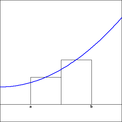
So far, we have used the simplest possible quadrilaterals (that is, rectangles) to estimate areas. It is natural, however, to wonder if other familiar shapes might serve us even better.
An alternative to \(L_n\text{,}\)\(R_n\text{,}\) and \(M_n\) is called the Trapezoid Rule. Rather than using a rectangle to estimate the (signed) area bounded by \(y = f(x)\) on a small interval, we use a trapezoid. For example, in Figure 4.2.8, we estimate the area under the curve using three subintervals and the trapezoids that result from connecting the corresponding points on the curve with straight lines.
Figure4.2.8.Estimating \(\int_a^b f(x) \ dx\) using three subintervals and trapezoids, rather than rectangles, where \(a = x_0\) and \(b = x_3\text{.}\)
The biggest difference between the Trapezoid Rule and a Riemann sum is that on each subinterval, the Trapezoid Rule uses two function values, rather than one, to estimate the (signed) area bounded by the curve. For instance, to compute \(D_1\text{,}\) the area of the trapezoid on \([x_0, x_1]\text{,}\) we observe that the left base has length \(f(x_0)\text{,}\) while the right base has length \(f(x_1)\text{.}\) The height of the trapezoid is \(x_1 - x_0 = \Delta x = \frac{b-a}{3}\text{.}\) The area of a trapezoid is the average of the bases times the height, so we have
Using similar computations for \(D_2\) and \(D_3\text{,}\) we find that \(T_3\text{,}\) the trapezoidal approximation to \(\int_a^b f(x) \, dx\) is given by
Because both left and right endpoints are being used, we recognize within the trapezoidal approximation the use of both left and right Riemann sums. Rearranging the expression for \(T_3\) by removing factors of \(\frac{1}{2}\) and \(\Delta x \text{,}\) grouping the left endpoint and right endpoint evaluations of \(f\text{,}\) we see that
We now observe that two familiar sums have arisen. The left Riemann sum \(L_3\) is \(L_3 = f(x_0) \Delta x + f(x_1) \Delta x + f(x_2) \Delta x\text{,}\) and the right Riemann sum is \(R_3 = f(x_1) \Delta x + f(x_2) \Delta x + f(x_3) \Delta x\text{.}\) Substituting \(L_3\) and \(R_3\) for the corresponding expressions in Equation (4.2.1), it follows that \(T_3 = \frac{1}{2} \left[ L_3 + R_3 \right]\text{.}\) We have thus seen a very important result: using trapezoids to estimate the (signed) area bounded by a curve is the same as averaging the estimates generated by using left and right endpoints.
The Trapezoid Rule.
The trapezoidal approximation, \(T_n\text{,}\) of the definite integral \(\int_a^b f(x) \, dx\) using \(n\) subintervals is given by the rule
In this activity, we explore the relationships among the errors generated by left, right, midpoint, and trapezoid approximations to the definite integral \(\int_1^2 \frac{1}{x^2} \, dx\text{.}\)
Use the First FTC to evaluate \(\int_1^2 \frac{1}{x^2} \, dx\) exactly.
Use appropriate computing technology to compute the following approximations for \(\int_1^2 \frac{1}{x^2} \, dx\text{:}\)\(T_4\text{,}\)\(M_4\text{,}\)\(T_8\text{,}\) and \(M_8\text{.}\)
Let the error that results from an approximation be the approximation’s value minus the exact value of the definite integral. For instance, if we let \(E_{T,4}\) represent the error that results from using the trapezoid rule with 4 subintervals to estimate the integral, we have
Based on your work in (a) and (b) above, compute \(E_{T,4}\text{,}\)\(E_{T,8}\text{,}\)\(E_{M,4}\text{,}\)\(E_{M,8}\text{.}\)
Which rule consistently over-estimates the exact value of the definite integral? Which rule consistently under-estimates the definite integral?
What behavior(s) of the function \(f(x) = \frac{1}{x^2}\) lead to your observations in (d)?
Subsection4.2.5Comparing the Midpoint and Trapezoid Rules
We know from the definition of the definite integral that if we let \(n\) be large enough, we can make any of the approximations \(L_n\text{,}\)\(R_n\text{,}\) and \(M_n\) as close as we’d like (in theory) to the exact value of \(\int_a^b f(x) \, dx\text{.}\) Thus, it may be natural to wonder why we ever use any rule other than \(L_n\) or \(R_n\) (with a sufficiently large \(n\) value) to estimate a definite integral. One of the primary reasons is that as \(n \to \infty\text{,}\)\(\Delta x = \frac{b-a}{n} \to 0\text{,}\) and thus in a Riemann sum calculation with a large \(n\) value, we end up multiplying by a number that is very close to zero. Doing so often generates roundoff error, because representing numbers close to zero accurately is a persistent challenge for computers.
Hence, we explore ways to estimate definite integrals to high levels of precision, but without using extremely large values of \(n\text{.}\) Paying close attention to patterns in errors, such as those observed in Activity 4.2.5, is one way to begin to see some alternate approaches.
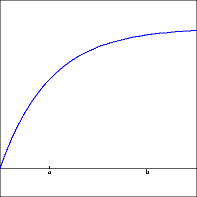
To begin, we compare the errors in the Midpoint and Trapezoid rules. First, consider a function that is concave up on a given interval, and picture approximating the area bounded on that interval by both the Midpoint and Trapezoid rules using a single subinterval.
Figure4.2.9.Estimating \(\int_a^b f(x) \ dx\) using a single subinterval: at left, the trapezoid rule; in the middle, the midpoint rule; at right, a modified way to think about the midpoint rule.
As seen in Figure 4.2.9, it is evident that whenever the function is concave up on an interval, the Trapezoid Rule with one subinterval, \(T_1\text{,}\) will overestimate the exact value of the definite integral on that interval. From a careful analysis of the line that bounds the top of the rectangle for the Midpoint Rule (shown in magenta), we see that if we rotate this line segment until it is tangent to the curve at the midpoint of the interval (as shown at right in Figure 4.2.9), the resulting trapezoid has the same area as \(M_1\text{,}\) and this value is less than the exact value of the definite integral. Thus, when the function is concave up on the interval, \(M_1\) underestimates the integral’s true value.
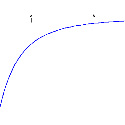
Figure4.2.10.Comparing the error in estimating \(\int_a^b f(x) \ dx\) using a single subinterval: in red, the error from the Trapezoid rule; in light red, the error from the Midpoint rule.
These observations extend easily to the situation where the function’s concavity remains consistent but we use larger values of \(n\) in the Midpoint and Trapezoid Rules. Hence, whenever \(f\) is concave up on \([a,b]\text{,}\)\(T_n\) will overestimate the value of \(\int_a^b f(x) \, dx\text{,}\) while \(M_n\) will underestimate \(\int_a^b f(x) \, dx\text{.}\) The reverse observations are true in the situation where \(f\) is concave down.
Next, we compare the size of the errors between \(M_n\) and \(T_n\text{.}\) Again, we focus on \(M_1\) and \(T_1\) on an interval where the concavity of \(f\) is consistent. In Figure 4.2.10, where the error of the Trapezoid Rule is shaded in red, while the error of the Midpoint Rule is shaded lighter red, it is visually apparent that the error in the Trapezoid Rule is more significant. To see how much more significant, let’s consider two examples and some particular computations.
If we let \(f(x) = 1-x^2\) and consider \(\int_0^1 f(x) \,dx\text{,}\) we know by the First FTC that the exact value of the integral is
Using appropriate technology to compute \(M_4\text{,}\)\(M_8\text{,}\)\(T_4\text{,}\) and \(T_8\text{,}\) as well as the corresponding errors \(E_{M,4}\text{,}\)\(E_{M,8}\text{,}\)\(E_{T,4}\text{,}\) and \(E_{T,8}\text{,}\) as we did in Activity 4.2.5, we find the results summarized in Table 4.2.11. We also include the approximations and their errors for the example \(\int_1^2 \frac{1}{x^2} \, dx\) from Activity 4.2.5.
Table4.2.11.Calculations of \(T_4\text{,}\)\(M_4\text{,}\)\(T_8\text{,}\) and \(M_8\text{,}\) along with corresponding errors, for the definite integrals \(\int_0^1 (1-x^2) \ dx\) and \(\int_1^2 \frac{1}{x^2} \ dx\text{.}\)
Rule
\(\int_0^1 (1-x^2) \,dx = 0.\overline{6}\)
error
\(\int_1^2 \frac{1}{x^2} \, dx = 0.5\)
error
\(T_4\)
\(0.65625\)
\(-0.0104166667\)
\(0.5089937642\)
\(0.0089937642\)
\(M_4\)
\(0.671875\)
\(0.0052083333\)
\(0.4955479365\)
\(-0.0044520635\)
\(T_8\)
\(0.6640625\)
\(-0.0026041667\)
\(0.5022708502\)
\(0.0022708502\)
\(M_8\)
\(0.66796875\)
\(0.0013020833\)
\(0.4988674899\)
\(-0.0011325101\)
For a given function \(f\) and interval \([a,b]\text{,}\)\(E_{T,4} = T_4 - \int_a^b f(x) \,dx\) calculates the difference between the approximation generated by the Trapezoid Rule with \(n = 4\) and the exact value of the definite integral. If we look at not only \(E_{T,4}\text{,}\) but also the other errors generated by using \(T_n\) and \(M_n\) with \(n = 4\) and \(n = 8\) in the two examples noted in Table 4.2.11, we see an evident pattern. Not only is the sign of the error (which measures whether the rule generates an over- or under-estimate) tied to the rule used and the function’s concavity, but the magnitude of the errors generated by \(T_n\) and \(M_n\) seems closely connected. In particular, the errors generated by the Midpoint Rule seem to be about half the size (in absolute value) of those generated by the Trapezoid Rule.
That is, we can observe in both examples that \(E_{M,4} \approx -\frac{1}{2} E_{T,4}\) and \(E_{M,8} \approx -\frac{1}{2}E_{T,8}\text{.}\) This property of the Midpoint and Trapezoid Rules turns out to hold in general: for a function of consistent concavity, the error in the Midpoint Rule has the opposite sign and approximately half the magnitude of the error of the Trapezoid Rule. Written symbolically,
This important relationship suggests a way to combine the Midpoint and Trapezoid Rules to create an even more accurate approximation to a definite integral.
Subsection4.2.6Simpson’s Rule
When we first developed the Trapezoid Rule, we observed that it is an average of the Left and Right Riemann sums:
If a function is always increasing or always decreasing on the interval \([a,b]\text{,}\) one of \(L_n\) and \(R_n\) will over-estimate the true value of \(\int_a^b f(x) \, dx\text{,}\) while the other will under-estimate the integral. Thus, the errors that result from \(L_n\) and \(R_n\) will have opposite signs; so averaging \(L_n\) and \(R_n\) eliminates a considerable amount of the error present in the respective approximations. In a similar way, it makes sense to think about averaging \(M_n\) and \(T_n\) in order to generate a still more accurate approximation.
We’ve just observed that \(M_n\) is typically about twice as accurate as \(T_n\text{.}\) So we use the weighted average
The rule for \(S_{2n}\) giving by Equation (4.2.2) is usually known as Simpson’s Rule. 4
Thomas Simpson was an 18th century mathematician; his idea was to extend the Trapezoid rule, but rather than using straight lines to build trapezoids, to use quadratic functions to build regions whose area was bounded by parabolas (whose areas he could find exactly). Simpson’s Rule is often developed from the more sophisticated perspective of using interpolation by quadratic functions.
Note that we use “\(S_{2n}\)” rather that “\(S_n\)” since the \(n\) points the Midpoint Rule uses are different from the \(n\) points the Trapezoid Rule uses, and thus Simpson’s Rule is using \(2n\) points at which to evaluate the function. We build upon the results in Table 4.2.11 to see the approximations generated by Simpson’s Rule. In particular, in Table 4.2.12, we include all of the results in Table 4.2.11, but include additional results for \(S_8 = \frac{2M_4 + T_4}{3}\) and \(S_{16} = \frac{2M_8 + T_8}{3}\text{.}\)
Table4.2.12.Table 4.2.11 updated to include \(S_8\text{,}\)\(S_{16}\text{,}\) and the corresponding errors.
Rule
\(\int_0^1 (1-x^2) \,dx = 0.\overline{6}\)
error
\(\int_1^2 \frac{1}{x^2} \, dx = 0.5\)
error
\(T_4\)
\(0.65625\)
\(-0.0104166667\)
\(0.5089937642\)
\(0.0089937642\)
\(M_4\)
\(0.671875\)
\(0.0052083333\)
\(0.4955479365\)
\(-0.0044520635\)
\(S_8\)
\(0.6666666667\)
\(0\)
\(0.5000298792\)
\(0.0000298792\)
\(T_8\)
\(0.6640625\)
\(-0.0026041667\)
\(0.5022708502\)
\(0.0022708502\)
\(M_8\)
\(0.66796875\)
\(0.0013020833\)
\(0.4988674899\)
\(-0.0011325101\)
\(S_{16}\)
\(0.6666666667\)
\(0\)
\(0.5000019434\)
\(0.0000019434\)
The results seen in Table 4.2.12 are striking. If we consider the \(S_{16}\) approximation of \(\int_1^2 \frac{1}{x^2} \, dx\text{,}\) the error is only \(E_{S,16} = 0.0000019434\text{.}\) By contrast, \(L_8 = 0.5491458502\text{,}\) so the error of that estimate is \(E_{L,8} = 0.0491458502\text{.}\) Moreover, we observe that generating the approximations for Simpson’s Rule is almost no additional work: once we have \(L_n\text{,}\)\(R_n\text{,}\) and \(M_n\) for a given value of \(n\text{,}\) it is a simple exercise to generate \(T_n\text{,}\) and from there to calculate \(S_{2n}\text{.}\) Finally, note that the error in the Simpson’s Rule approximations of \(\int_0^1 (1-x^2) \, dx\) is zero! 5
Similar to how the Midpoint and Trapezoid approximations are exact for linear functions, Simpson’s Rule approximations are exact for quadratic and cubic functions. See additional discussion on this issue later in the section and in the exercises.
These rules are not only useful for approximating definite integrals such as \(\int_0^1 e^{-x^2} \, dx\text{,}\) for which we cannot find an elementary antiderivative of \(e^{-x^2}\text{,}\) but also for approximating definite integrals when we are given a function through a table of data.
Activity4.2.6.
A car traveling along a straight road is braking and its velocity is measured at several different points in time, as given in the following table. Assume that \(v\) is continuous, always decreasing, and always decreasing at a decreasing rate, as is suggested by the data.
seconds, \(t\)
Velocity in ft/sec, \(v(t)\)
\(0\)
\(100\)
\(0.3\)
\(99\)
\(0.6\)
\(96\)
\(0.9\)
\(90\)
\(1.2\)
\(80\)
\(1.5\)
\(50\)
\(1.8\)
\(0\)
Table4.2.13.Data for the braking car.
Figure4.2.14.Axes for plotting the data in Activity 4.2.3.
Plot the given data on the set of axes provided in Figure 4.2.14 with time on the horizontal axis and the velocity on the vertical axis.
What definite integral will give you the exact distance the car traveled on \([0,1.8]\text{?}\)
Estimate the total distance traveled on \([0,1.8]\) by computing \(L_3\text{,}\)\(R_3\text{,}\) and \(T_3\text{.}\) Which of these under-estimates the true distance traveled?
Estimate the total distance traveled on \([0,1.8]\) by computing \(M_3\text{.}\) Is this an over- or under-estimate? Why?
Using your results from (c) and (d), improve your estimate further by using Simpson’s Rule.
What is your best estimate of the average velocity of the car on \([0,1.8]\text{?}\) Why? What are the units on this quantity?
Subsection4.2.7Overall observations regarding \(L_n\text{,}\)\(R_n\text{,}\)\(T_n\text{,}\)\(M_n\text{,}\) and \(S_{2n}\text{.}\)
As we conclude our discussion of numerical approximation of definite integrals, it is important to summarize general trends in how the various rules over- or under-estimate the true value of a definite integral, and by how much. To revisit some past observations and see some new ones, we consider the following activity.
Activity4.2.7.
Consider the functions \(f(x) = 2-x^2\text{,}\)\(g(x) = 2-x^3\text{,}\) and \(h(x) = 2-x^4\text{,}\) all on the interval \([0,1]\text{.}\) For each of the questions that require a numerical answer in what follows, write your answer exactly in fraction form.
On the three sets of axes provided in Figure 4.2.15, sketch a graph of each function on the interval \([0,1]\text{,}\) and compute \(L_1\) and \(R_1\) for each. What do you observe?
Compute \(M_1\) for each function to approximate \(\int_0^1 f(x) \,dx\text{,}\)\(\int_0^1 g(x) \,dx\text{,}\) and \(\int_0^1 h(x) \,dx\text{,}\) respectively.
Compute \(T_1\) for each of the three functions, and hence compute \(S_2\) for each of the three functions.
Evaluate each of the integrals \(\int_0^1 f(x) \,dx\text{,}\)\(\int_0^1 g(x) \,dx\text{,}\) and \(\int_0^1 h(x) \,dx\) exactly using the First FTC.
For each of the three functions \(f\text{,}\)\(g\text{,}\) and \(h\text{,}\) compare the results of \(L_1\text{,}\)\(R_1\text{,}\)\(M_1\text{,}\)\(T_1\text{,}\) and \(S_2\) to the true value of the corresponding definite integral. What patterns do you observe?
Figure4.2.15.Axes for plotting the functions in Activity 4.2.4.
The results seen in Activity 4.2.7 generalize nicely. For instance, if \(f\) is decreasing on \([a,b]\text{,}\)\(L_n\) will over-estimate the exact value of \(\int_a^b f(x) \,dx\text{,}\) and if \(f\) is concave down on \([a,b]\text{,}\)\(M_n\) will over-estimate the exact value of the integral. An excellent exercise is to write a collection of scenarios of possible function behavior, and then categorize whether each of \(L_n\text{,}\)\(R_n\text{,}\)\(T_n\text{,}\) and \(M_n\) is an over- or under-estimate.
Finally, we make two important notes about Simpson’s Rule. When T. Simpson first developed this rule, his idea was to replace the function \(f\) on a given interval with a quadratic function that shared three values with the function \(f\text{.}\) In so doing, he guaranteed that this new approximation rule would be exact for the definite integral of any quadratic polynomial. In one of the pleasant surprises of numerical analysis, it turns out that even though it was designed to be exact for quadratic polynomials, Simpson’s Rule is exact for any cubic polynomial: that is, if we are interested in an integral such as \(\int_2^5 (5x^3 - 2x^2 + 7x - 4)\, dx\text{,}\)\(S_{2n}\) will always be exact, regardless of the value of \(n\text{.}\) This is just one more piece of evidence that shows how effective Simpson’s Rule is as an approximation tool for estimating definite integrals. 6
One reason that Simpson’s Rule is so effective is that \(S_{2n}\) benefits from using \(2n+1\) points of data. Because it combines \(M_n\text{,}\) which uses \(n\) midpoints, and \(T_n\text{,}\) which uses the \(n+1\) endpoints of the chosen subintervals, \(S_{2n}\) takes advantage of the maximum amount of information we have when we know function values at the endpoints and midpoints of \(n\) subintervals.
Subsection4.2.8Summary
A Riemann sum is simply a sum of products of the form \(f(x_i^*) \Delta x\) that estimates the area between a positive function and the horizontal axis over a given interval. If the function is sometimes negative on the interval, the Riemann sum estimates the difference between the areas that lie above the horizontal axis and those that lie below the axis.
The three most common types of Riemann sums are left, right, and middle sums, but we can also work with a more general Riemann sum. The only difference among these sums is the location of the point at which the function is evaluated to determine the height of the rectangle whose area is being computed. For a left Riemann sum, we evaluate the function at the left endpoint of each subinterval, while for right and middle sums, we use right endpoints and midpoints, respectively.
The left, right, and middle Riemann sums are denoted \(L_n\text{,}\)\(R_n\text{,}\) and \(M_n\text{,}\) with formulas
\begin{align*}
L_n = f(x_0) \Delta x + f(x_1) \Delta x + \cdots + f(x_{n-1}) \Delta x \amp= \sum_{i = 0}^{n-1} f(x_i) \Delta x,\\
R_n = f(x_1) \Delta x + f(x_2) \Delta x + \cdots + f(x_{n}) \Delta x \amp= \sum_{i = 1}^{n} f(x_i) \Delta x,\\
M_n = f(\overline{x}_1) \Delta x + f(\overline{x}_2) \Delta x + \cdots + f(\overline{x}_{n}) \Delta x \amp= \sum_{i = 1}^{n} f(\overline{x}_i) \Delta x\text{,}
\end{align*}
where \(x_0 = a\text{,}\)\(x_i = a + i\Delta x\text{,}\) and \(x_n = b\text{,}\) using \(\Delta x = \frac{b-a}{n}\text{.}\) For the midpoint sum, \(\overline{x}_{i} = (x_{i-1} + x_i)/2\text{.}\)
The Trapezoid Rule, which estimates \(\int_a^b f(x) \, dx\) by using trapezoids, rather than rectangles, can also be viewed as the average of Left and Right Riemann sums. That is, \(T_n = \frac{1}{2}(L_n + R_n)\text{.}\)
The Midpoint Rule is typically twice as accurate as the Trapezoid Rule, and the signs of the respective errors of these rules are opposites. Hence, by taking the weighted average \(S_{2n} = \frac{2M_n + T_n}{3}\text{,}\) we can build a much more accurate approximation to \(\int_a^b f(x) \, dx\) by using approximations we have already computed. The rule for \(S_{2n}\) is known as Simpson’s Rule, which can also be developed by approximating a given continuous function with pieces of quadratic polynomials.
Exercises4.2.9Exercises
1.Evaluating Riemann sums for a quadratic function.
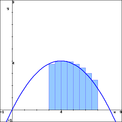
The rectangles in the graph below illustrate a left endpoint Riemann sum for \(\displaystyle f(x) = \frac{-x^{2}}{4}+2x\) on the interval \(\lbrack 3, 7 \rbrack\text{.}\)
The value of this left endpoint Riemann sum is , and this Riemann sum is
[select an answer]
an overestimate of
equal to
an underestimate of
there is ambiguity
the area of the region enclosed by \(\displaystyle y = f(x)\text{,}\) the x-axis, and the vertical lines x = 3 and x = 7.
Left endpoint Riemann sum for \(y = \frac{-x^{2}}{4}+2x\) on \(\lbrack 3, 7 \rbrack\)
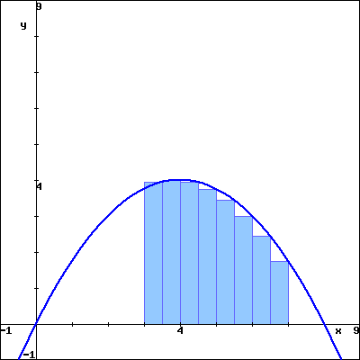
The rectangles in the graph below illustrate a right endpoint Riemann sum for \(\displaystyle f(x) = \frac{-x^{2}}{4}+2x\) on the interval \(\lbrack 3, 7 \rbrack\text{.}\)
The value of this right endpoint Riemann sum is , and this Riemann sum is
[select an answer]
an overestimate of
equal to
an underestimate of
there is ambiguity
the area of the region enclosed by \(\displaystyle y = f(x)\text{,}\) the x-axis, and the vertical lines x = 3 and x = 7.
Right endpoint Riemann sum for \(y = \frac{-x^{2}}{4}+2x\) on \(\lbrack 3, 7 \rbrack\)
2.Estimating distance traveled with a Riemann sum from data.
Your task is to estimate how far an object traveled during the time interval \(0 \leq t \leq 8\text{,}\) but you only have the following data about the velocity of the object.
time (sec)
0
1
2
3
4
5
6
7
8
velocity (feet/sec)
-4
-2
-3
1
2
3
2
3
4
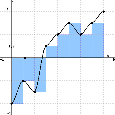
To get an idea of what the velocity function might look like, you pick up a black pen, plot the data points, and connect them by curves. Your sketch looks something like the black curve in the graph below.
Left endpoint approximation
You decide to use a left endpoint Riemann sum to estimate the total displacement. So, you pick up a blue pen and draw rectangles whose height is determined by the velocity measurement at the left endpoint of each one-second interval. By using the left endpoint Riemann sum as an approximation, you are assuming that the actual velocity is approximately constant on each one-second interval (or, equivalently, that the actual acceleration is approximately zero on each one-second interval), and that the velocity and acceleration have discontinuous jumps every second. This assumption is probably incorrect because it is likely that the velocity and acceleration change continuously over time. However, you decide to use this approximation anyway since it seems like a reasonable approximation to the actual velocity given the limited amount of data.
(A) Using the left endpoint Riemann sum, find approximately how far the object traveled. Your answers must include the correct help (units) 7
/pg_files/helpFiles/Units.html
.
Total displacement =
Total distance traveled =
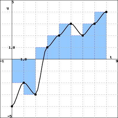
Using the same data, you also decide to estimate how far the object traveled using a right endpoint Riemann sum. So, you sketch the curve again with a black pen, and draw rectangles whose height is determined by the velocity measurement at the right endpoint of each one-second interval.
Right endpoint approximation
(B) Using the right endpoint Riemann sum, find approximately how far the object traveled. Your answers must include the correct help (units) 8
/pg_files/helpFiles/Units.html
.
Total displacement =
Total distance traveled =
3.Writing basic Riemann sums.
On a sketch of \(y = e^{x}\text{,}\) represent the left Riemann sum with \(n = 2\) approximating \(\int_{0}^{1}\,e^{x}\,dx\text{.}\) Write out the terms of the sum, but do not evaluate it:
Sum = +
On another sketch, represent the right Riemann sum with \(n = 2\) approximating \(\int_{0}^{1}\,e^{x}\,dx\text{.}\) Write out the terms of the sum, but do not evaluate it:
Sum = +
Which sum is an overestimate?
the left Riemann sum
the right Riemann sum
neither sum
Which sum is an underestimate?
the right Riemann sum
the left Riemann sum
neither sum
4.
Consider the function \(f(x) = 3x + 4\text{.}\)
Compute \(M_4\) for \(y=f(x)\) on the interval \([2,5]\text{.}\) Be sure to clearly identify the value of \(\Delta x\text{,}\) as well as the locations of \(x_0, x_1, \ldots, x_4\text{.}\) Include a careful sketch of the function and the corresponding rectangles being used in the sum.
Use a familiar geometric formula to determine the exact value of the area of the region bounded by \(y = f(x)\) and the \(x\)-axis on \([2,5]\text{.}\)
Explain why the values you computed in (a) and (b) turn out to be the same. Will this be true if we use a number different than \(n = 4\) and compute \(M_n\text{?}\) Will \(L_4\) or \(R_4\) have the same value as the exact area of the region found in (b)?
Describe the collection of functions \(g\) for which it will always be the case that \(M_n\text{,}\) regardless of the value of \(n\text{,}\) gives the exact net signed area bounded between the function \(g\) and the \(x\)-axis on the interval \([a,b]\text{.}\)
Assume that \(S\) is a right Riemann sum. For what function \(f\) and what interval \([a,b]\) is \(S\) this function’s Riemann sum? Why?
How does your answer to (a) change if \(S\) is a left Riemann sum? a middle Riemann sum?
Suppose that \(S\) really is a right Riemann sum. What is geometric quantity does \(S\) approximate?
Use sigma notation to write a new sum \(R\) that is the right Riemann sum for the same function, but that uses twice as many subintervals as \(S\text{.}\)
6.
A car traveling along a straight road is braking and its velocity is measured at several different points in time, as given in the following table.
Table4.2.22.Data for the braking car.
seconds, \(t\)
\(0\)
\(0.3\)
\(0.6\)
\(0.9\)
\(1.2\)
\(1.5\)
\(1.8\)
Velocity in ft/sec, \(v(t)\)
\(100\)
\(88\)
\(74\)
\(59\)
\(40\)
\(19\)
\(0\)
Plot the given data on a set of axes with time on the horizontal axis and the velocity on the vertical axis.
Estimate the total distance traveled during the car the time brakes using a middle Riemann sum with 3 subintervals.
Estimate the total distance traveled on \([0,1.8]\) by computing \(L_6\text{,}\)\(R_6\text{,}\) and \(\frac{1}{2}(L_6 + R_6)\text{.}\)
Assuming that \(v(t)\) is always decreasing on \([0,1.8]\text{,}\) what is the maximum possible distance the car traveled before it stopped? Why?
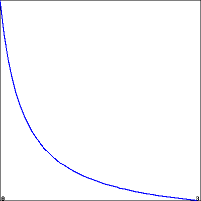
7.
The rate at which pollution escapes a scrubbing process at a manufacturing plant increases over time as filters and other technologies become less effective. For this particular example, assume that the rate of pollution (in tons per week) is given by the function \(r\) that is pictured in Figure 4.2.23.
Use the graph to estimate the value of \(M_4\) on the interval \([0,4]\text{.}\)
What is the meaning of \(M_4\) in terms of the pollution discharged by the plant?
Suppose that \(r(t) = 0.5 e^{0.5t}\text{.}\) Use this formula for \(r\) to compute \(L_5\) on \([0,4]\text{.}\)
Determine an upper bound on the total amount of pollution that can escape the plant during the pictured four week time period that is accurate within an error of at most one ton of pollution.
Figure4.2.23.The rate, \(r(t)\text{,}\) of pollution in tons per week.
8.Comparison of methods for increasing concave down function.
Using the figure showing \(f(x)\) below, order the following approximations to the integral \(\int_0^3\,f(x)\,dx\) and its exact value from smallest to largest.
(Click on the graph for a larger version.)
Enter each of "LEFT(n)", "RIGHT(n)", "TRAP(n)", "MID(n)" and "Exact" in one of the following answer blanks to indicate the correct ordering:
\(\lt \)\(\lt \)\(\lt \)\(\lt \)
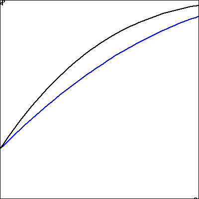
9.Comparing accuracy for two similar functions.
Using a fixed number of subdivisions, we approximate the integrals of \(f\) and \(g\) on the interval shown in the figure below.
(The function \(f(x)\) is shown in blue, and \(g(x)\) in black; click on the graph to get a larger version.)
For which function, \(f\) or \(g\) is LEFT more accurate?
\(\displaystyle f\)
\(\displaystyle g\)
For which function, \(f\) or \(g\) is RIGHT more accurate?
\(\displaystyle f\)
\(\displaystyle g\)
For which function, \(f\) or \(g\) is MID more accurate?
\(\displaystyle f\)
\(\displaystyle g\)
For which function, \(f\) or \(g\) is TRAP more accurate?
\(\displaystyle f\)
\(\displaystyle g\)
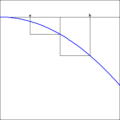
10.Identifying and comparing methods.
Consider the four functions shown below. On the first two, an approximation for \(\int_a^b\,f(x)\,dx\) is shown.
1.
2.
3.
4.
(Click on any graph to get a larger version.)
1. For graph number 1, Which integration method is shown?
midpoint rule
trapezoid rule
right rule
left rule
Is this method an over- or underestimate?
over
under
2. For graph number 2, Which integration method is shown?
midpoint rule
trapezoid rule
left rule
right rule
Is this method an over- or underestimate?
over
under
3. On a copy of graph number 3, sketch an estimate with \(n=2\) subdivisions using the left rule.
Is this method an over- or underestimate?
under
over
4. On a copy of graph number 4, sketch an estimate with \(n=2\) subdivisions using the trapezoid rule.
Is this method an over- or underestimate?
under
over
11.
Consider the definite integral \(\int_0^1 x \tan(x) \, dx\text{.}\)
Explain why this integral cannot be evaluated exactly by using either \(u\)-substitution or by integrating by parts.
Using appropriate subintervals, compute \(L_4\text{,}\)\(R_4\text{,}\)\(M_4\text{,}\)\(T_4\text{,}\) and \(S_8\text{.}\)
Which of the approximations in (b) is an over-estimate to the true value of \(\int_0^1 x \tan(x) \, dx\text{?}\) Which is an under-estimate? How do you know?
12.
For an unknown function \(f(x)\text{,}\) the following information is known.
\(f\) is continuous on \([3,6]\text{;}\)
\(f\) is either always increasing or always decreasing on \([3,6]\text{;}\)
\(f\) has the same concavity throughout the interval \([3,6]\text{;}\)
As approximations to \(\int_3^6 f(x) \, dx\text{,}\)\(L_4 = 7.23\text{,}\)\(R_4 = 6.75\text{,}\) and \(M_4 = 7.05\text{.}\)
Is \(f\) increasing or decreasing on \([3,6]\text{?}\) What data tells you?
Is \(f\) concave up or concave down on \([3,6]\text{?}\) Why?
Determine the best possible estimate you can for \(\int_3^6 f(x) \, dx\text{,}\) based on the given information.
13.
The rate at which water flows through Table Rock Dam on the White River in Branson, MO, is measured in cubic feet per second (CFS). As engineers open the floodgates, flow rates are recorded according to the following chart.
Table4.2.24.Water flow data.
seconds, \(t\)
\(0\)
\(10\)
\(20\)
\(30\)
\(40\)
\(50\)
\(60\)
flow in CFS, \(r(t)\)
\(2000\)
\(2100\)
\(2400\)
\(3000\)
\(3900\)
\(5100\)
\(6500\)
What definite integral measures the total volume of water to flow through the dam in the 60 second time period provided by the table above?
Use the given data to calculate \(M_n\) for the largest possible value of \(n\) to approximate the integral you stated in (a). Do you think \(M_n\) over- or under-estimates the exact value of the integral? Why?
Approximate the integral stated in (a) by calculating \(S_n\) for the largest possible value of \(n\text{,}\) based on the given data.
Compute \(\frac{1}{60} S_n\) and \(\frac{2000+2100+2400+3000+3900+5100+6500}{7}\text{.}\) What quantity do both of these values estimate? Which is a more accurate approximation?